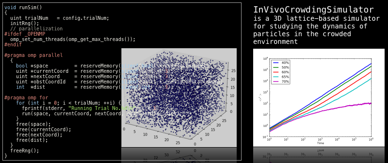
InVivoCrowdingSimulator: A 3D lattice-based simulator for studying the dynamics of particles in the crowded environment.
Latest release: 1.0.0, released 5th May 2012
Overview
InVivoCrowdingSimulator (IVCSim) is a 3D lattice-based simulator for studying the dynamics of particles in the crowded environment (like in vivo environment). The simulator outputs MSD (Mean Square Displacement) corresponding to the time. The simulator uses "Blind Ant model" for Brownian motion. The library should build and work without serious troubles on Unix based operating systems (Linux, MacOSX and FreeBSD).
Download
InVivoCrowdingSimulator is distributed under the terms of LGPL.
- Source code (in tar + gzipped format) invivosim-1.0.0.tar.gz
Dependencies
InVivoCrowdingSimulator (IVCSim) requires the GNU Scientific Library (GSL) which is a numerical library to be installed on your system. Please follow the instruction on GSL webpage and install GSL. If you have multi-core system (such as Core2Duo, Core2Quad, Core i5, Core i7, Phenome X4, etc.) and want to improve the performance of your simulation, compiling IVCSim with OpenMP might be your help.
Installation
IVCSim is written in C99, thus it should build and work without serious troubles on Unix based operating systems (Linux, MacOSX and FreeBSD). We have tested IVCSim to work on Linux and MacOSX, both with and without OpenMP.
How to build IVCSim
- Extract the archive file
- Compile
tar xvzf invivosim-1.0.0.tar.gz
cd invivosim-1.0.0/
vim Makefile  (edit Makefile with your favorite editor)
modify CFLAGS and LDFLAGS to correctly find your GSL. By default, compiler will try to find the header files and libraries under /usr, /usr/local and /opt/local directories. This might work on most of the UNIX based operating systems. If your system have OpenMP, then you can enable it by uncommenting following 2 lines:
#OMPINC = -fopenmp
#OMPLIB = -lgomp
By using OpenMP, simulation will be automatically parallelized results to performance improvement. Finally, type 'make' and compilation will start.
make
Usage
Following files will be generated by the compilation.
- msd_in_fixed_obstacles
3D lattice-based simulator with "fixed" obstacles in reaction space. The obstacles will not move during the simulation. The size of each obstacle is just as the same size of a lattice. Single molecule (particle) will be dropped in the reaction space, and move during the simulation. The simulation result will be achieved as the Mean Square Displacement (MSD) of the particle.- Runtime Arguments:
arg.1: lattice size (> 0)
arg.2: max steps (> 0)
arg.3: obstacle rate (>= 0.0 and < 1.0)
arg.4: trial number (> 0)
- Example:
./msd_in_fixed_obstacles 30 1000 0.3 100Reaction space is 30*30*30(arg.1) with 30%(arg.3) of obstacles. Let one particle move in the space until 1,000 time steps(arg.2), Iterate this simulation for 100 times(arg.4), and then calculate average MSD for each time points.
3D lattice-based simulator with "moving" obstacles in reaction space. The obstacles will move with the specified duration. The size of each obstacle is just as the same size of a lattice. Single molecule (particle) will be dropped in the reaction space, and move during the simulation. The simulation result will be achieved as the Mean Square Displacement (MSD) of the particle.
- Runtime Arguments:
arg.1: lattice size (> 0)
arg.2: max steps (> 0)
arg.3: obstacle rate (>= 0.0 and < 1.0)
arg.4: trial number (> 0)
arg.5: obstacle moving interval
./msd_fix_to_move_obstacles 30 1000 0.3 100 5Reaction space is 30*30*30(arg.1) with 30%(arg.3) of obstacles. Obstacles will move in every 5 time steps(arg.5). Let one particle move in the space until 1,000 time steps(arg.2), Iterate this simulation for 100 times(arg.4), and then calculate average MSD for each time points.
3D lattice-based simulator with "moving" obstacles in reaction space. The obstacles will move with the specified duration. The size of each obstacle (sphere) can be specified with this simulator. Each obstacle has its volume, so that the simulator takes care that the obstacles will not placed on other obstacle. Single molecule (particle) will be dropped in the reaction space, and move during the simulation. The simulation result will be achieved as the Mean Square Displacement (MSD) of the particle.
- Runtime Arguments:
arg.1: lattice size (> 0)
arg.2: max steps (> 0)
arg.3: obstacle radius
arg.4: obstacle rate (>= 0.0 and < 1.0)
arg.5: obstacle moving interval
arg.6: trial number (> 0)
./msd_in_move_sphere 30 1000 2 0.3 100 5Reaction space is 30*30*30(arg.1) with 30%(arg.4) of obstacles. The radius of obstacle is 2 (arg.3). Obstacles will move in every 5 time steps(arg.5). Let one particle move in the space until 1,000 time steps(arg.2), Iterate this simulation for 100 times(arg.6), and then calculate average MSD for each time points.
This is just a support application to visualize the reaction space. With given arguments, this program will dump the reaction space in to a file "space.txt", which describes the position of all obstacles in the reaction space. Each line contains x, y and z position of each obstacle. You can visualize the reaction space with following python script (visualize_space.py)
- Runtime Arguments:
arg.1: lattice size (> 0)
arg.2: obstacle rate (>= 0.0 and < 1.0)
./dump_space 30 0.4Reaction space is 30*30*30(arg.1) with 40%(arg.2) of obstacles. The reaction space will be dumped to a file "space.txt".
This python script will visualize the reaction space generated by the above program dump_space. To run this script, you have to install matplotlib, which is a python plotting library. This script will simply reads "space.txt" and generate a 3D plot. You can save the visualized reaction space as PDF, PNG file from the graphical user interface.
- Example:
./dump_space 30 0.2 && python visualize_space.pyReaction space of 30*30*30(arg.1) with 20%(arg.2) of obstacles will be displayed as 3D plot.
Authors
InVivoCrowdingSimulator has been primary developed by
- Keisuke Iba
with substantial contributions from
- Akito Tabira
- Takeshi Kubojima
- Noriko Hiroi
- Akira Funahashi
Contact
If you have any questions / comments, please send an email to
InVivoCrowdingSimulator development team: <info_at_fun.bio.keio.ac.jp> (please replace _at_ with @)
We appreciate your feedback!
Funding acknowledgements
This work have been supported by the following organizations: SUNTORY Institute for Bioorganic Research (Japan) and Keio University (Japan).
News
- 2021-12-15: Akira Funahashi was invited to deliver talk at the JBRAIC (日本乳腺人工知能研究会). His talk title was "深層学習と医学研究(in Japanese)".
- 2021-10-19: A paper entitled: "COVID19 Disease Map, a computational knowledge repository of virus–host interaction mechanisms" is published in Molecular Systems Biology.
- 2021-10-15: Our paper entitled: "SBMLWebApp: Web-Based Simulation, Steady-State Analysis, and Parameter Estimation of Systems Biology Models" by Takahiro G. Yamada et al. is published in MDPI Processes.
- 2021-10-05: A paper entitled: "Cas9-mediated genome editing reveals a significant contribution of calcium signaling pathways to anhydrobiosis in Pv11 cells" is published in Scientific Reports.
- 2021-08-07: Akira Funahashi was invited to deliver talk at the Japanese Society for Quantitative Biology Summer 2021. His talk title was "機械学習と定量生物学(in Japanese)".
- 2021-05-28: A paper entitled: "Genome-Wide Role of HSF1 in Transcriptional Regulation of Desiccation Tolerance in the Anhydrobiotic Cell Line, Pv11" is published in International Journal of Molecular Sciences.
- 2021-03-23: Akira Funahashi was invited to deliver talk at the Data Driven Biology Workshop. His talk title was "深層学習が駆動する定量生物学の新展開(in Japanese)".
- 2021-02-11: Takahiro Yamada was invited to deliver talk at the The 40th Scienc-ome. His talk title was "限界を超えた能力を生命に付与したい ー設計図志向な生物学を目指してー (in Japanese)".
- 2021-01-27: Our research on QCANet has been featured in SigOpt's blog.
- 2020-12-14: The book on Machine Learning and Life Sciences "機械学習を生命科学に使う!" was published.
- 2020-11-06: Our research results on QCANet were published in Asahi Newspaper. "AI analysis may lead to improved chance of success of IVF pregnancy : The Asahi Shimbun".
- 2020-10-19: The research project on Mathematical Information Platform, in which we are participating as co-researchers, has been accepted by the funding program JST CREST.
- 2020-10-10: Yuta Tokuoka was awarded the Best Poster Award at the Society of Reproductive Biology for Young Scientists(第7回 生殖若手の会).
- 2020-10-05: Akira Funahashi was invited to deliver keynote speech at the "Computational Modeling in Biology" Network (COMBINE) 2020. His talk title was "CellDesigner: A modeling tool for biochemical networks".
- 2020-09-22: Ryo Nakatani was invited to deliver talk at 2020 Japanese Society for Mathematical Biology annual meeting (JSMB 2020, 2020年度 日本数理生物学会年会). His talk title was "一細胞系譜解析による低グルコース培養下大腸菌集団のATP濃度多様性の解明 (in Japanese)".
- 2020-09-15: Our paper entitled: "Direct cell counting using macro-scale smartphone images of cell aggregates" by Chikahiro Imashiro, Yuta Tokuoka et al. is published in IEEE Access.
- 2020-09-09: Akira Funahashi was invited to deliver talk at The 81st Japan Society of Applied Physics Autumun Meeting 2020(第81回 応用物理学会 秋季学術講演会). His talk title was "ライブセルイメージングと深層学習を用いた 胚発生過程定量システムの構築 (in Japanese)".
- 2020-08-26: A paper entitled: "SBML Level 3: an extensible format for the exchange and reuse of biological models" is published in Molecular Systems Biology.
- 2020-05-05: A paper entitled: "COVID-19 Disease Map, building a computational repository of SARS-CoV-2 virus-host interaction mechanisms" is published in Scientific Data.
- 2020-03-19: Our paper entitled: "Identification of a master transcription factor and a regulatory mechanism for desiccation tolerance in the anhydrobiotic cell line Pv11" by Takahiro Yamada et al. is published in PLOS ONE.
- 2020-03-13: The book (Cell Biology by the Numbers) we translated was published (数でとらえる細胞生物学).
- 2020-02-03: Our paper entitled: "Neural Differentiation Dynamics Controlled by Multiple Feedback Loops in a Comprehensive Molecular Interaction Network" by Tsuyoshi Iwasaki et al. is published in MDPI Processes.
- 2019-12-14: Our paper entitled: "Deep Learning for Non-Invasive Determination of the Differentiation Status of Human Neuronal Cells by Using Phase-Contrast Photomicrographs" by Maya Ooka et al. is published in MDPI Applied Sciences.
- 2019-11-07: Akira Funahashi was invited to deliver talk at 群馬大学総合外科学講座 Translational Researchセミナー. His talk title was "人工知能と医学研究(in Japanese)".
- 2019-11-07: Ryo Nakatani was selected to deliver talk at Quantitative Biology Japan Caravan 2019(定量生物学の会 北海道キャラバン 2019). His talk title was "一細胞系譜による低グルコース培養下大腸菌集団のATP濃度多様性生成機構の解明(in Japanese)".
- 2019-10-22: Our paper entitled: "XitoSBML: A Modeling Tool for Creating Spatial Systems Biology Markup Language Models From Microscopic Images" by Kaito Ii et al. is published in Frontiers in Genetics.
- 2019-10-18: Our review article entitled: "Development of 3D imaging system with an electrically tunable lens (in Japanese)" by Akira Funahashi et al. is published in Experimental Medicine (実験医学).
- 2019-09-05: Akira Funahashi was invited to deliver talk at 群馬大学数理データ科学教育研究センター主催第1回レギュラトリーサイエンスセミナー. His talk title was "腫瘍内不均一性を考慮した予後の予測に向けた 深層学習ベースの組織画像解析(in Japanese)".
- 2019-09-05: Our paper entitled: "Predicting the future direction of cell movement with convolutional neural networks" by Shori Nishimoto et al. is published in PLOS ONE.
- 2019-08-29: Yuta Tokuoka and Akira Funahashi were invited to deliver talk at Grant-in-Aid for Scientific Research on Innovative Areas- Platforms for Advanced Technologies and Research Resources "Advanced Bioimaging Support(ABiS)" Training Course (新学術領域研究・学術研究支援基盤形成 「先端バイオイメージング支援プラットフォーム」AIによる生物画像解析トレーニングコース). Their talk title was "機械学習による画像分類(in Japanese)".
- 2019-07-17: Akira Funahashi was invited to deliver talk at COMBINE 2019. His talk title was "CellDesigner: A modeling tool for biochemical networks".
- 2019-07-01: Our review article entitled: "Basis for diagnosis using image analysis and deep learning (in Japanese)" by Akira Funahashi et al. is published in Pathology and Clinical Medicine (病理と臨床).
- 2019-05-28: Akira Funahashi was invited to deliver talk at AI Systems Medicine Research and Training Center, Yamaguchi University. His talk title was "畳み込みニューラルネットワークを用いた神経分化判別および特徴量解析(in Japanese)".
- 2019-05-20: CellDesigner version 4.4.2 released! CellDesigner is a modeling tool of biochemical networks.
- 2019-05-20: Akira Funahashi was invited to deliver talk at Cardiovascular Meeting, Keio University School of Medicine. His talk title was "Deep Learning-based Quantitative Evaluation of Early Embryo in Fertility Treatments Perspective (in Japanese)".
- 2019-03-08: Shori Nishimoto was invited to deliver talk at School of Veterinary Medicine and Science, University of Nottingham. His talk title was "Deep Learning Based Tissue Analysis for Predicting Cancer Outcomes Accounting for Intratumoral Heterogeneity".
- 2019-03-08: Akira Funahashi was invited to deliver talk at School of Veterinary Medicine and Science, University of Nottingham. His talk title was "Convolutional Neural Network-Based Instance Segmentation Algorithm to Acquire Quantitative Criteria of Early Mouse Development".
- 2019-03-06: Our paper entitled: "Activation of cell migration via morphological changes in focal adhesions depends on shear stress in MYCN-amplified neuroblastoma cells" by Takumi Hiraiwa et al. is published in Journal of the Royal Society Interface.
- 2019-02-26: Yuta Tokuoka was invited to deliver talk at Engineering Network Workshop - Fusion of tolerance function of life and engineering -. His talk title was "深層学習が駆動するPv11生存細胞スクリーニング(in Japanese)".
- 2019-02-22: Mikiko Motomuro was selected to deliver talk at The Seventh Annual Winter Q-bio meeting. Her talk title was "Mechanical Modeling of Cell Migration During the Early Embryogenesis of C. elegans to Reveal the Mechanism for Controlling Cell Arrangement".
- 2019-02-21: Takayuki Nakamura was selected to deliver talk at The Seventh Annual Winter Q-bio meeting. His talk title was "Analysis of Intracellular Temperature Effect on Wound Healing Process".
- 2018-12-18: Our paper entitled: "Transcriptome analysis of the anhydrobiotic cell line Pv11 infers the mechanism of desiccation tolerance and recovery" by Takahiro G Yamada et al. is published in Scientific Reports.
- 2018-12-14: Akira Funahashi was invited to deliver talk at AI Systems Medicine Research and Training Center, Yamaguchi University. His talk title was "深層学習が明らかにする細胞顕微鏡画像解析の新展開(in Japanese)".
- 2018-09-21: Noriko Hiroi was invited to deliver talk at Keio University International Symposium on Advanced Technologies for Mechano-biology and Regenerative Medicine. Her talk title was "Quantitative analysis of sensitivity to Wnt3a gradient in determination of the pole-to-pole axis of mitotic cells by using a microfluidic device".
- 2018-09-16: Our paper entitled: "Quantitative analysis of sensitivity to a Wnt3a gradient in determination of the pole‐to‐pole axis of mitotic cells by using a microfluidic device" by Takumi Hiraiwa et al. is published in FEBS Open Bio.
- 2018-09-14: Takahiro Yamada was selected to deliver talk at SICE Annual Conference 2018 (SICE 2018). His talk title was "Mathematical Modeling Identifies the Conditions Required for RNA-Based Oscillator".
- 2018-09-13: Yoshitaka Yamazaki was selected to deliver talk at 2nd Keio Life Science Symposium. He also received a research encouragement award! His talk title was "In silico 及び in vivo 実験による有糸分裂期中心体位置制御機構の解明(in Japanese)".
- 2018-09-06: Takahiro G Yamada was invited to deliver talk at CELLab-SOCU Summer Symposium. His talk title was "カラカラに乾燥しても死なないネムリユスリカの神秘に転写制御ネットワークから迫る(in Japanese)".
- 2018-07-27: Akira Funahashi was invited to deliver talk at The 36th Annual Meeting of Japan Society of Fertilization and Implantation. His talk title was "ディープラーニングを用いたマウス発生過程における定量的指標の獲得(in Japanese)".
- 2018-07-17: Akira Funahashi was invited to deliver talk at 関西医科大学大学院. (in Japanese)
- 2018-05-23: Takahiro Yamada was invited to deliver talk at Life of Genomes 2018. His talk title was "Inferring a Polypedilum vanderplanki transcriptional regulatory network for rehydration process from time-series RNA-seq data".
- 2018-03-15: Akira Funahashi was invited to deliver talk at 自然科学研究機構新分野創成センター合同シンポジウム 「分野横断・分野融合研究による生命創成を探究する新しい科学の創成」. His talk title was "深層学習が明らかにする細胞顕微鏡画像解析の新展開(in Japanese)".
- 2018-03-01: Akira Funahashi was invited to deliver talk at SYSBIO 2018 Advanced Lecture Course on Systems Biology. His talk title was "CellDesigner: A process diagram editor for gene-regulatory and biochemical networks".
- 2017-12-05: LibSBMLSim version 1.4.0 released! LibSBMLSim enables you to write your own SBML capable simulator with a few lines of code.
- 2017-08-11: Yuta Tokuoka was selected to deliver talk at 18th International Conference on Systems Biology (ICSB 2017). His talk title was "Segmenting four-dimensional fluorescence microscopic image using Convolutional Neural Network".
- 2017-06-23: Noriko Hiroi was invited to deliver talk at EMERGING RESEARCH CHALLENGES IN BIOLOGY. Her talk title was "Asymmetric division, cell migration, and differentiation control in microfluidic devices".
- 2017-06-20: Noriko Hiroi was invited to deliver talk at EMN Europe Meeting on Quantum. Her talk title was "The foundation of Biothermology from the point of view of nano/microscale thermophysical properties of biopolymers".
- 2017-04-24: Noriko Hiroi was invited to deliver talk at Biomedical Imaging and Sensing Conference. Her talk title was "Requirement of spatiotemporal resolution for imaging intracellular temperature distribution".
- 2017-01-08: Yuta Tokuoka was selected to deliver talk at 8th Annual workshop on Quantitative Biology Japan (定量生物学の会 第8回年会). His talk title was "深層学習を用いた3次元蛍光顕微鏡画像セグメンテーションアルゴリズムの提案(in Japanese)".
- 2016-12-14: Matthew Higashionna is invited to deliver talk at International Symposium on Micro-Nano Science and Technology 2016 (MNST 2016). His talk title will be "Quantification of the effect of shear stress on the differentiation of SH-SY5Y cells".
- 2016-05-27: Our editorial article entitled: "Quantitative Biology: Dynamics of living systems" by Noriko Hiroi et al. is published in Frontiers in Physiology (Systems Biology).
- 2016-03-01: Our paper entitled: "Detection of Temperature Difference in Neuronal Cells" by Ryuichi Tanimoto et al. is published in Scientific Reports.
- 2016-02-10: A review entitled: "Simulation technology and its application in Systems Biology (in Japanese)" by Akira Funahashi and Noriko Hiroi. is published in Folia Pharmacologica Japonica.
- 2015-06-24: A review entitled: "The principles of whole-cell modeling" by Jonathan R Karr et al. is published in Current Opinion in Microbiology.
- 2015-05-26: A review entitled: "Bioimage Analysis for Quantitative Biology and Its Application to Mammalian Embryogenesis (in Japanese)" by Tetsuya J Kobayashi et al. is published in Medical Imaging Technology.
- 2015-02-13: Our paper entitled: "Acceleration of discrete stochastic biochemical simulation using GPGPU" by Kei Sumiyoshi et al. is published in Frontiers in Physiology (Systems Biology).
- 2015-01-21: Our paper entitled: "High-speed microscopy with an electrically tunable lens to image the dynamics of in vivo molecular complexes" by Yuichiro Nakai et al. is published in Review of Scientific Instruments.
- 2015-01-16: A paper entitled: "A proteomic study of mitotic phase-specific interactors of EB1 reveals a role for SXIP-mediated protein interactions in anaphase onset" is published in Biology Open.
- 2014-07-16: A book chapter entitled: "Modeling and simulation using CellDesigner" is published in Methods in Molecular Biology.
- 2014-04-04: Our paper entitled: "Assessing uncertainty in model parameters based on sparse and noisy experimental data" by Noriko Hiroi et al. is published in Frontiers in Physiology (Systems Biology).
- 2013-08-23: A paper entitled: "Automated tracking of mitotic spindle pole positions shows that LGN is required for spindle rotation but not orientation maintenance" is published in Cell Cycle.
- 2013-07-05: A paper entitled: "The systems biology simulation core algorithm" is published in BMC Systems Biology.
- 2013-07-04: Noriko Hiroi was invited to deliver talk at The 35th Annual International Conference of the IEEE Engineering in Medicine and Biology Society (EMBC’13). Her talk title was "In Vivo Oriented Modeling with Consideration of Intracellular Crowding".
- 2013-06-28: Akira Funahashi was invited to deliver talk on CellDesigner at The 2nd HD Physiology International Symposium.
- 2013-05-07: Akira Funahashi and Noriko Hiroi were invited to organize a two days workshop on CellDesigner at Monash University, Australia.
- 2013-04-05: Our paper entitled: "LibSBMLSim: a reference implementation of fully functional SBML simulator" by Hiromu Takizawa et al. is published in Bioinformatics.
- 2013-01-28: LibSBMLSim version 1.1.0 released! LibSBMLSim enables you to write your own SBML capable simulator with a few lines of code.
- 2012-12-20: Our paper entitled: "Mathematical Modeling of Sustainable Synaptogenesis by Repetitive Stimuli Suggests Signaling Mechanisms In Vivo" by Noriko Hiroi and Hiromu Takizawa is published in PLoS ONE.
- 2012-12-07: A General Commentary Article entitled: "Meeting Report of the International Workshop on Quantitative Biology 2012: Mesoscopic and microscopic worlds meet." by Viji M. Draviam et al. is published in Frontiers in Physiology (Systems Biology).
- 2012-11-25: We had "5th Annual Meeting of The Japanese Society for Quantitative Biology (Q-BioJP)" at the University of Tokyo.
- 2012-11-22: We had "International Workshop on Quantitative Biology 2012" at the University of Tokyo.
- 2012-07-23: Our paper entitled: "Physiological intracellular crowdedness is defined by the perimeter-to-area ratio of sub-cellular compartments" by Noriko Hiroi is published in Frontiers in Fractal Physiology.
- 2012-06-26: Our paper entitled: "From Microscopy Data to in silico Environments for in vivo Oriented Simulations" by Noriko Hiroi is published in EURASIP Journal on Bioinformatics and Systems Biology.
- 2012-05-10: A paper entitled: "Software support for SBGN maps: SBGN-ML and LibSBGN" by Martijn P. van Iersel et al. is published in Bioinformatics.
- 2012-04-04: LibSBMLSim version 1.0.0 released! LibSBMLSim enables you to write your own SBML capable simulator with a few lines of code.
- 2011-10-21: A paper entitled: "BioPAX support in CellDesigner" by Huaiyu Mi et al. is published in Bioinformatics.
- 2011-09-15: Our paper is taken up on a Japanese news site.
- 2011-03-13: A paper entitled: "Physiological environment induce quick response - slow exhaustion reactions" by Noriko Hiroi is published in Frontiers in Physiology (Systems Biology).
Contact information
Funahashi Lab.
Room 516, 520C, 520I and 417, Bld 14,
Department of Biosciences and Informatics,
Keio University,
3-14-1 Hiyoshi
Kouhoku-ku, Yokohama
223-8522 JAPAN
Phone: +81-45-566-1797
Email: info _at_ fun.bio.keio.ac.jp